
Evaluating College Volleyball Rankings
This article will talk about the process of web scraping, cleaning, and evaluating college volleyball statistics for athletes in the Big 10 Conference in 2023.
Introduction
Watching volleyball is one of my favorite pastimes. Seeing how each team reacts and which players seem to dominate the court has always been fascinating. But there is always the question of what makes a good player? Is it their hitting skill, how hard they serve, or how many times they pass the ball? We will be exploring these questions and much more.
The first thing to do is to get a data set with player rankings. To do this we will be using the Big 10 Conference volleyball player rankings from 2023. First we will look into web scraping the data, and ethics behind it. Then we will organize it and see what information we can get from it.
Ethics of Web Scraping
Before Web Scraping any website, you should check the robots.txt file. This can be found on almost any website; all you have to do is type in the url/robots.txt. The robots.txt file tells each type of bot what part of the website they are allowed to scrap and how they should go about scraping it. These are some examples of robots.txt files:
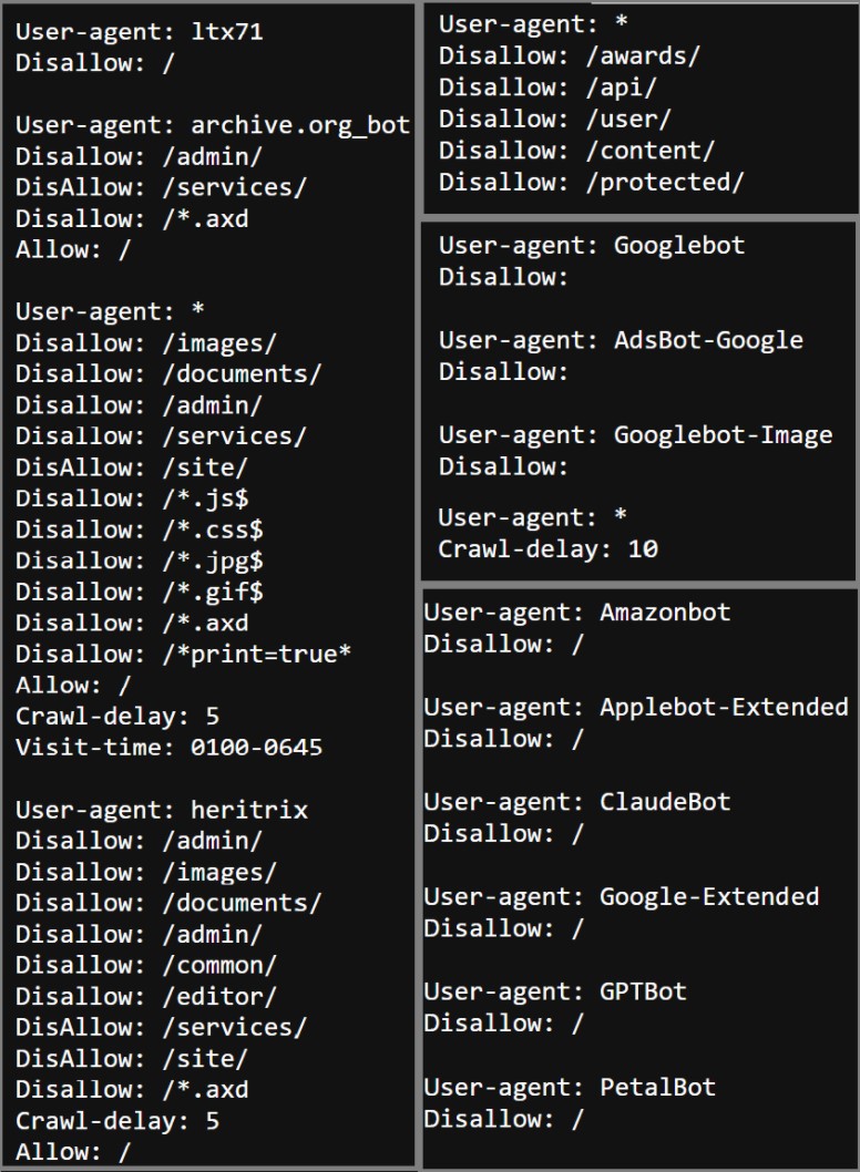
These files show different bots names and what they are allowed to scrap and not allowed scrap by each type of bot. For the general user you need to look at the bot file indicated with an astrix (*). Along with where you are allowed to scrap, the file can also have some restrictions on how often you can make requests, shown by the ‘Crawl-delay:’, what hours you can scrap it, and other restrictions. You can find more information on web scraping here.
The Robots.txt file for the Big 10 website does not restrict any of the pages from being web scrapped. It also doesen’t indicate a crawl speed. So we can web scrap this site with no limitations.
Web Scraping
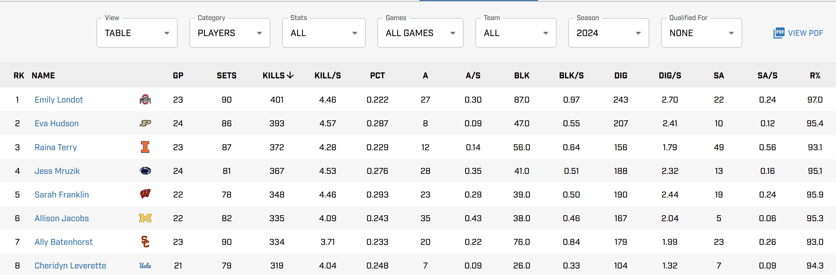
For this example, we will be looking at the website for the Big 10 Conference volleyball teams. The first thing that we needed to do is make sure that all of the required packages are installed. The packages that we will be using to do this project are pandas, selenium, webdriver-manager, and beautifulsoup4. Each of these packages have important functions that are vital for webscrapping. This particular website. The table we will be scrapping from is shown below. As you can see there are several buttons along the top that you can use to see different statistics or seasons. We will need to use these to get the data we want.
First, we need to set up the driver. To do this we use the webdriver function found in selenium. I will be using a Chrome driver, however, depending on your browser you may need to use a different function. How to do this is shown in the code below.
url = 'https://bigten.org/wvb/stats/'
driver = webdriver.Chrome(service=ChromeService(ChromeDriverManager().install()))
driver.get(url)
As mentioned above we will need to use the buttons along the top of the screen to get the data we want. We want to scrap from the 2023 season but he default for the website is 2024. To change this, we will need to use another special feature in selenium that allows us to click on items on the webpage. First, the website needs to be completely loaded, for this we will use the WebDriverWait funtion. Then we will click the area that shows the season. Next, we will tell it which year to select and then click on it. If you want to look at different years you can just change where it says 2023 to be the year you would like to look at.
wait = WebDriverWait(driver, 10)
dropdown = wait.until(EC.element_to_be_clickable((By.ID, "stats-select-season")))
dropdown.click()

year_option = driver.find_element(By.XPATH, ".//li[text()='2023']")
year_option.click()
If you would like more information on selenium you can find it here.
Now that we have the appropriate table, we want to use the package beautiful soup to get the html and information from the table. Using the following code, we create the beautiful soup object and get the table.
soup = BeautifulSoup(driver.page_source, 'html.parser')
table = soup.find('table')
We can use the find and find all commands from the beautiful soup package to first get the headers from the table. These will be the names of all the variables we will be looking at.
headers = []
head = table.find('thead')
all = head.find_all('th')

for row in all:
    name = row.find('div').text
    headers.append(name)
Next, we need to get the row information from the table. We will use the same functions of find and find_all within a for loop to get all the values.
body = table.find('tbody')
rows = []
for row in body.find_all('tr'):
    data = []
    for item in row.find_all('td'):
        thing = item.text
        data.append(thing)
    rows.append(data)
Finally, we will use the pandas package to create a data frame with all the information from the table in it.
data2023 = pd.DataFrame(rows, columns= headers)
Be sure to close the driver when you have finished scraping the data by using the driver.close function.
If you would like to learn more about using the BeautifulSoup packages click here
Data Cleaning
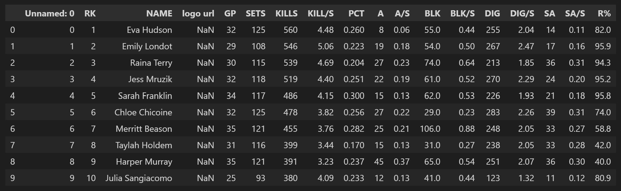
The next step is to make sure that we can use the data that we got from website. Luckily in this case the data is already pretty clean. This is what the first few rows of data will look like right after web scraping.
Getting rid of unwanted columns is our first priority. The two columns we want to remove are the ‘Unnamed: 0’ and ‘logo url’. To do this we will use the drop function found in the pandas package. We use the columns option in drop and put in a list of the columns we would like to remove. We will also use the rename function to change the column names to be more descriptive of the variable. An example of these two functions are shown below.
players = players2023.drop(columns= ['Unnamed: 0', 'logo url'])
players = players.rename(columns= {'RK' : 'rank', 'NAME':'name','GP':'games_played',
                            'SETS':'sets_played','KILLS': 'kills', 'KILL/S':'kills_per_set',
                            'PCT': 'hitting_percentage', 'A':'assists', 'A/S': 'assists_per_set',
                            'BLK':'blocks', 'BLK/S':'blocks_per_set', 'DIG':'digs',
                            'DIG/S':'digs_per_set', 'SA':'service_aces',
                            'SA/S':'service_aces_per_set', 'R%':'reception_percentage'})
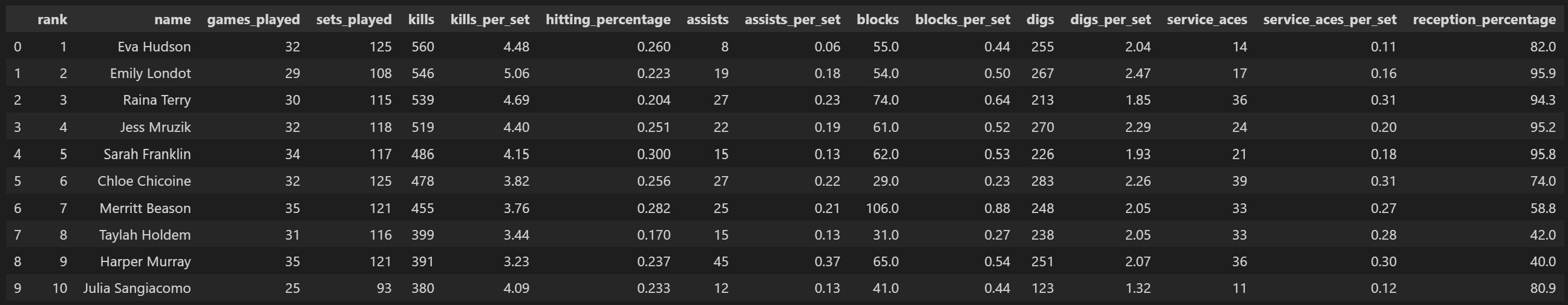
The data frame should now look like this:
Exploring the Data
Finally, we can look into different trends in the data and what it tells us about highly ranked players. One interesting way we can look at this is by the correlation matrix of each of the variables. We do this through the matplotlib package and the seaborn package.
Because the name, and the number of games or sets played do not tell us much about the ranking we will be removing them from the correlation matrix. While looking at the matrix it is important to remember that the highest rank is 1, making a lot of the correlations negative.
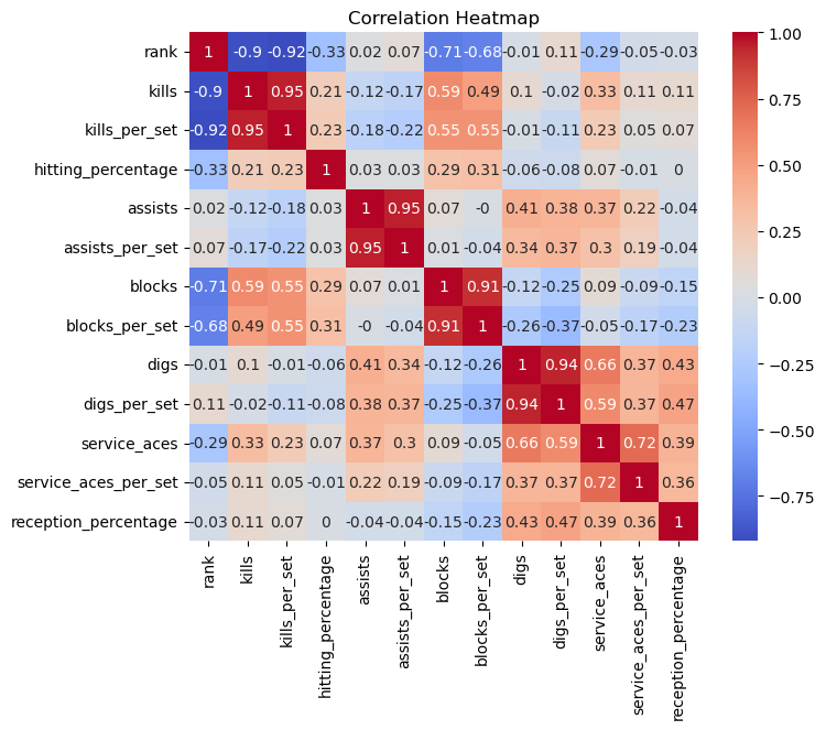
There are a few interesting trends shown in the correlation matrix:
- Kills and Kill per Set are correlated with the Rank A kill is scoring a point off of a hit
- Blocks and Blocks per Set are correlated with Rank Blocks are when teams stop someone from hitting over the net and it comes back on hitters side
- Blocks and Kills are correlated with each other
- Service Aces and Digs are correlated * Digs are passing a hard driven ball well and services aces are when the server gets a point from serving
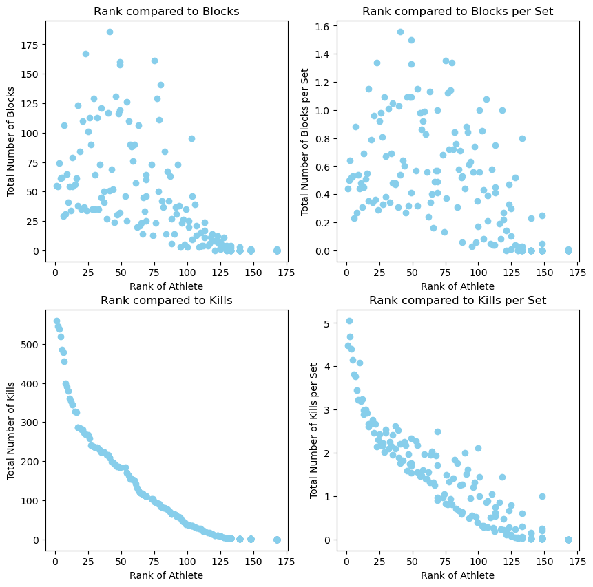
We can compare each of these correlations through scatterplots. As you can see, when the rank is closer to 1 the athletes tend to have more kills and more blocks. This shows us that the players with the highest rankings tend to be front row players.
The code for all of the following plots can be found in the github repository at the end of the post.
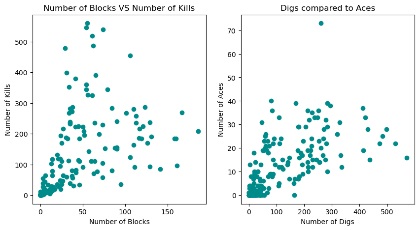
We can also compare blocks to kills and aces to digs in a scatterplots.
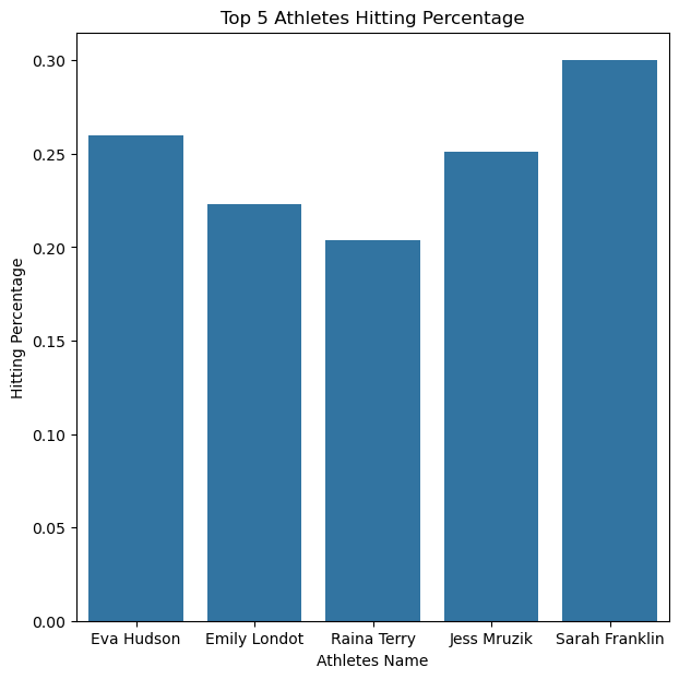
Another interesting thing to look at is the stats by the athlete’s name. We can do this by using a bar graph. In this graph it shows the top five highest ranked players hitting percentages. They all have a fairly high hitting percentage, making them challenging players to defend.
Learn more about seaborn and matplotlib
Conclusion
In conclusion, through the graphics it was made clear that the players who had more hits and blocks were more likely to appear higher in the rankings than those who were lower. However, we barely scraped the tip of the iceberg of possibilities for this data. We talked about how to webscrap and what to pay attention to in robots.txt files. We covered how to select the columns we need and rename them. And then we showed some different visualizations we can use to display the data. Now that you have done this for the volleyball data set, you can do it for any data set that you can find. Go and find a data set that interests you and see what you can uncover!
You can access all of the code in the github repository by clicking here.